rjsf

License

MIT + file LICENSE

Citation

Authors

Thanh Long Vu (author, maintainer, copyright holder)
Domenic Germano (author)
Michael Lydeamore (author)

rjsf provides an R interface to Jump-Switch-Flow (JSF), a hybrid simulation framework for compartmental models that combines stochastic jump dynamics at low populations with deterministic flow dynamics at high populations.

Important: rjsf is an R interface; running simulations requires the Python Jump-Switch-Flow backend to be installed and accessible through reticulate.

The main function is jsf_simulate(), which lets users define compartmental reaction models in R and return simulation output as either a regular data.frame or a structured JSFResult object.

Installation

Once available on CRAN, you can install the released version of rjsf with:

install.packages("rjsf")

You can install the development version from GitHub with:

# install.packages("pak")
pak::pak("olivervu25/rjsf")

Python setup

rjsf uses reticulate to call the Python jsf package. This means Python jsf must be installed in the same Python environment that reticulate is using.

A recommended setup is to create a local virtual environment:

python3 -m venv .venv
source .venv/bin/activate

python -m pip install --upgrade pip setuptools wheel
python -m pip install numpy scipy pandas matplotlib python-libsbml
python -m pip install git+https://github.com/DGermano8/jsf

Then in R, point reticulate to that environment:

Sys.setenv(RETICULATE_PYTHON = ".venv/bin/python")

library(reticulate)
py_config()

Check that Python jsf is available:

library(rjsf)

jsf_available()

This should return:

[1] TRUE

Alternative setup using reticulate

You can also install the Python dependencies from R using reticulate:

library(reticulate)

virtualenv_create("rjsf-env")

py_install(
  packages = c("numpy", "scipy", "pandas", "matplotlib", "python-libsbml"),
  envname = "rjsf-env",
  method = "virtualenv"
)

py_install(
  packages = "git+https://github.com/DGermano8/jsf",
  envname = "rjsf-env",
  method = "virtualenv",
  pip = TRUE
)

use_virtualenv("rjsf-env", required = TRUE)

Then check:

library(rjsf)

jsf_available()

Quick example

The following example simulates a Lotka-Volterra predator-prey system and returns a structured JSFResult object.

library(rjsf)
library(reticulate)

rates_lv <- reticulate::py_eval(
  "lambda x, t: [2.0 * x[0], 1.5 * x[1], 0.05 * x[0] * x[1]]"
)

result <- jsf_simulate(
  x0 = c(prey = 50, predator = 10),
  rates = rates_lv,
  reactant = matrix(
    c(
      1, 0,
      0, 1,
      1, 1
    ),
    ncol = 2,
    byrow = TRUE
  ),
  product = matrix(
    c(
      2, 0,
      0, 0,
      0, 2
    ),
    ncol = 2,
    byrow = TRUE
  ),
  do_disc = c(1, 1),
  t_max = 10,
  dt = 0.01,
  switching_threshold = c(30, 30),
  species_names = c("prey", "predator"),
  return_type = "JSFResult"
)

result
summary(result)
plot(result)

Output types

jsf_simulate() can return either a regular data frame:

df <- jsf_simulate(..., return_type = "data.frame")

or a structured JSFResult object:

result <- jsf_simulate(..., return_type = "JSFResult")

A JSFResult stores simulation trajectories and metadata, and supports:

print(result)
summary(result)
plot(result)

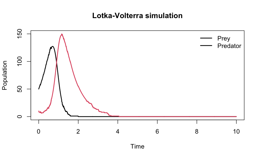
The simulated prey and predator trajectories can be visualised directly from the JSFResult object:

Lotka-Volterra prey and predator trajectories generated with rjsf

Vignettes

See the getting started vignette for full Lotka-Volterra and SIR examples.

Links